Formatting Cells in Excel For A Better Understanding Of Information

Different colors, a new font, wider columns, borderlines: Formatting cells in Excel can help make the information easier to understand. In our previous lesson (Excel Spreadsheet Basics Everyone Should Know About), we introduced the parts of a spreadsheet and how to move around. Now let’s format our cells, rows, and columns.

Formatting Cells in Excel | Easy Information Breakdown

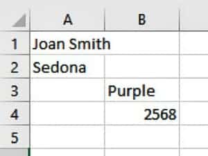
Open up a blank Excel spreadsheet and type your name in Cell A1, your city in Cell A2, and your favorite color in Cell B3. In Cell B4, type the number “2568.” Notice that the words will all “align” or line up to the left side of each cell, and the number will “align” to the right.

To format a cell, first, you must select the cell. It doesn’t matter if you have information in the cell or it is blank. The formatting you assign will be assigned to that cell until you change it.

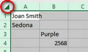
Let’s “Select All” by clicking the small box between Column A and Row 1. You can also “Select All” by pressing Ctrl-A. Remember, there is usually more than one correct way to give a command.

Font

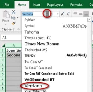
Now that you’ve selected “All,” pick a different font from the Home tab>Font section drop-down menu. Scroll down near the bottom and select the Verdana font. Verdana was created by an engineer to be easily read in spreadsheets, both letters, and numbers. For example, the numbers “6” and “8” are very distinct. Did you notice that when you hovered your mouse over “Verdana” the spreadsheet was previewing the new font? Try it again and point to different fonts. You’ll see what it looks like before you click one. Hit “Esc” to leave Verdana as the chosen font.

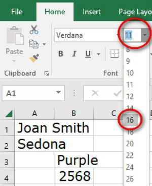
Boldface, italics, underline and font size are all available on the “Home tab>Font” section. Still with “Select All,” click the “Home tab>Font section>Font Size” drop-down arrow to get the font size menu. Hover your mouse over the bigger numbers. Do you see the rows and columns getting bigger, too? Excel knows that bigger fonts need more room. Increase the font size from 11 to 16. We’ll talk about row height and column width below.

Fill Color and Font Color

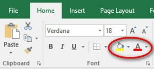
Within the Home tab>Font section are cell colors and font colors. Do you see that little paint bucket icon in the Home tab>Font section? This is the Fill Color icon, and it usually defaults to yellow. Select Column B by clicking the letter “B,” then use the little paint bucket icon to “fill” in the cells with your favorite color. To pick purple, I’ll go to the “Home tab>Font section>click on the Fill Color” drop-down arrow, then select purple. You pick your favorite, and all of Column B is now your favorite color.

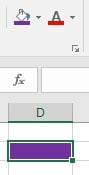
Notice that the Fill Color “bucket” will remember the last color you used until you change it. Click on Cell D2, then click the Fill Color bucket without touching the drop-down arrow, and the cell will turn your favorite color.

When you use dark colors, it is difficult to read black letters, so we will change the letters to white inside the purple cells. If you selected a light color, just turn them white anyway. To select just the two purple cells with black letters, drag through Cells B3 and B4. Click the “Home tab>Font section>Font Color” drop-down arrow next to the “A” with the colored underline. Select the color white from the palette.

Your favorite color now fills the cell and the letters are white. Experiment with the colors until you find a combination that is easy to read.

Column Width and Row Height

Does some of your name from Cell A1 run into Cell B1? Excel does that on purpose. If there is nothing inside the cell to the right, it allows one cell to overlap the next.

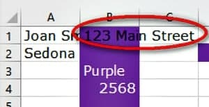
Go into Cell B1 and type your address with both the number and street. Quite a few things happened here that I want to bring to your attention.

Your street address wrote over Cell B1 and covered up the last part of your name.

Your street address is still in black lettering since we only changed the font color for Cells B3 and B4.

Excel didn’t right-align your address even though it started with a number. If I had just typed “123” the cell would have aligned to the right. As soon as I typed a letter, Excel recognized the entry as text and aligned it to the left.

Hopefully, that gives you an idea of how Excel thinks and behaves.

Let’s give your name a little more room. Hover your cursor between the “A” and “B” column headings, and it will change into the “Stretch” cursor, a vertical line with left and right arrows. Click on the line between “A” and “B” and drag the column width to the right two or three inches.

Oops, that’s probably too far. Instead of dragging this time, double-click the little vertical line between the “A” and “B.” Double-clicking the column divider tells Excel to make the column just big enough for the largest entry in Column A. That largest entry is your name, so now your entire name is showing. Row height works exactly the same way, except your drag or double-click the little horizontal line between the “1” and “2.”

Practice the skills in the Cells Color and Font Color you learned to change the cell and font color of your address.

Borders

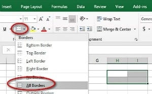
Select a group of four blank cells, two down and two across, then pick the Home tab>Font section>Borders drop-down arrow. Click on “All Borders” from the menu, and a thin black line will outline all four cells in the group.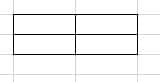

Borders can be a bit confusing, so experiment with “All Borders” and “No Borders” then just the right and left. You can make the lines thicker or dotted by choosing Line Style from the Border drop-down menu. For custom and even diagonal lines, you may select the last item, “More Borders.” This takes some practice, so play now before you need it in a rushed, high-stress situation.

Experiment and Clear Formatting

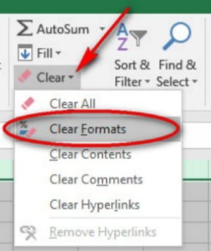
Formatting cells in Excel takes some practice so let’s start over by clearing all this formatting. Select All with “Ctrl-A” or by clicking that box between Column A and Row 1. In the “Home tab>Editing section>click the Clear” drop-down arrow. From the Clear drop-down menu, click on “Clear Formats.” This will leave your cell contents but return to Excel’s default font, size, and colors.

Now that you have a blank slate, experiment with the “Home tab>Font” section.

 

Have you tried formatting cells in excel recently? Let us know how it went in the comments section below.

Up Next: How to Use Microsoft Excel for First Timers | Easy Comprehensive Guide