Excel Formulas and Dollar Format

Curious to learn more about Excel formulas? Spreadsheets can help users find instant results when making calculations. For example, let’s say we are selling fruit at a local Farmer’s Market. Excel could help us calculate the total price if shoppers buy more than one of each item. Before trying this lesson, feel free to brush up on the basics of Excel if needed. You can find a short introduction in “Excel Spreadsheet Basics” and “Excel Formatting Cells.”

Excel Formulas and Dollar Format

Enter the Information

Let’s create a little spreadsheet. Use Tab to move one cell to the right, and Enter to move one cell down. Start in Cell A1, and make headings for your columns. Then you’ll add some fruit and prices.

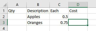
Your spreadsheet should look like this when you are finished entering the data. Always enter one bit of information in each cell before moving to the next cell – don’t just hit the space bar, use Tab, Enter or your cursor keys. When you are entering the prices, you don’t need to enter a “leading zero” in the dollar place. Just type “.5” for fifty cents and “.75” for seventy-five cents.

Dollar Format

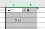
Both the “Each” price and the “Cost” price are dollar amounts. Correct formatting will line up the decimal points in fifty cents and seventy-five cents. Click on Column C above “Each” then hold down the mouse button until you get to Column D above “Cost.” Are both columns selected?

Since Excel helps us with numbers, there are shortcuts to most common number formats in the:

Home tab>Number section

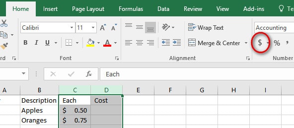
We want a dollar sign and two decimal points, so after selecting Columns C and D, click:

Home tab>Number section>$

Each price is now in dollar format, and the numbers line up properly. This same formatting will apply to any number or sum we enter in either Column C or Column D.

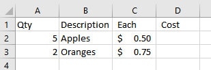
Let’s add how many apples and oranges we sold. We sold five apples, so to the left of Apples, in Cell A2, type “5” and press Enter to go down to Cell A3. We sold two oranges, so enter that. Notice that numbers always align to the right edge of the cell, and text always aligns to the left. Your table should look like this now.

Create a Formula

There are four basic arithmetic operations in Excel formulas:

+ addition
– subtraction
* multiplication
/ division

Find each of these characters on your keyboard or the number keypad, along with the equals sign “=” which begins every Excel formula.

Add Two Cells

We will add our quantities together to see how many pieces of fruit we sold today.

Go to Cell A4 and press “=” to begin our formula. We are adding Cell A2 to Cell A3, so we could type “=A2+A3” but it is much easier to have Excel put in the cell names for you.

After you type “=,” click on Cell A2. Excel will fill that in for you. Now type the plus and click on Cell A3. Don’t press Enter yet!

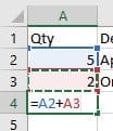
The formula “=A2+A3” will appear in both the Formula Bar and inside Cell A4. Notice the colors. While you are typing the formula, Excel gives each cell and “cell reference” name a color so you can check your work. Look over your formula then press Enter to save it inside Cell A4.

Let’s say the customer just came back and wanted one more orange. Go to Cell A3 and type “3” and press Enter. What happened to our total in Cell A4? It immediately adjusted our total to eight pieces of fruit! Make sure your spreadsheet shows “8.”

Multiply Two Cells

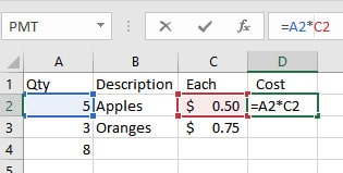
We want Excel to calculate the cost of each type of fruit. Click on Cell D2, right under the word “Cost.” Start with the equals sign, then click on the quantity of apples, Cell A2.

For multiplication, type the asterisk. Now click on the price each, Cell C2. Your formula is Cell D2 should be “=A2*C2,” right?

Check the formula for the helpful colors, and press Enter if it’s correct. The colors disappear when I press Enter, but if I go back to Cell D2 and click anywhere on the Formula Bar, the colors reappear to help me make any changes or “edit” my formula.

Copy and Paste Formulas | Relative Reference

We could enter our formula again on Row 3 for our oranges, but let’s copy and paste instead. Click on Cell D2 and right-click Copy or Ctrl-C. Now click on Cell D3 and right-click Paste or Ctrl-V. The cost of the oranges is $2.25. Excel did not copy the cost or “value” inside the Cell D2, it copied the formula, so our answer is specific to the oranges. With your cursor on Cell D3, click on the Formula Bar and read those cell references.

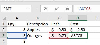
When Excel pasted the formula, it made a slight change. The new equation is on Row 3, so Instead of multiplying numbers on Row 2, it changed all the cell references to Row 3. The copied formula is now “=A3*C3.” That is a very important concept in Excel.

When it copies formulas, it keeps the numbers “relative” to their row or column. The opposite of “relative” is “absolute” which is another lesson for another day.

Let’s change a number to test both our formulas. Change the number of apples to 10. Your total quantity changes to “13” and your cost of apples changes to $5.00.

Sum Formula

In our Quantity column, we added two numbers, but what if there were rows and rows of data? Instead of clicking on each individual row when we create our addition formula, we can get a “sum” of a group or “range” of numbers with the “=SUM()” formula.

Excel will even write it for us. Look at the right side of the Home tab and you will see an “Autosum” icon in the Editing section, the Greek letter Sigma (∑).

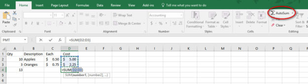
Click on Cell D4 at the bottom of our cost column. Now click on the Home tab>Editing section>Autosum. Excel writes in the formula and guesses that you want to sum the range of numbers from Cell D2 to Cell D3. Excel always puts the range in parenthesis with a colon between (D2:D3).

Excel is also using its colors and drawing a dotted line around the range. Sometimes Excel guesses correctly and something it doesn’t – so it waits for you to give the okay. This time it is correct, so press Enter.

Save this simple spreadsheet as “Excel Practice.” We will use it again to create a table.

Was this lesson helpful? Let us know in the comments section below!

Up Next: How To Use Microsoft Online | Important Notes You Need To Know