Excel Table | How To Format Excel Tables with Total Sort and Filter
 Want to edit your own Excel Table? A worksheet, even if it is full of data like dates and number formats, can still gain from improvements. A change in custom format, the use of the format painter or conditional formatting here and there, or a simple addition of linestyle can do wonders for an excel worksheet or excel file. In this lesson we’ll discuss how to create and format a table, edit the cells, sort and filter it.
How To Format and Edit Excel Tables
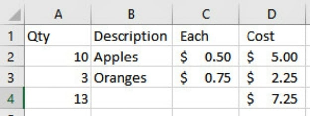
Follow along! In this template we’ll be using the same excel spreadsheet we made in our last lesson. Recreate or open this simple spreadsheet from our last lesson: Excel Formulas.
Show Formulas
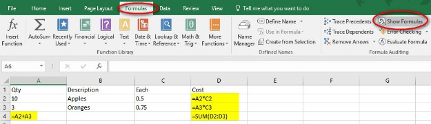
Do your formulas match the sample? There is a quick way to check. Click on Formulas tab and in the drop-down menu, go for Formula Auditing section>Show Formulas. To go back to normal, just click “Show Formulas” again; it’s an on/off button.
Insert Copied Cells
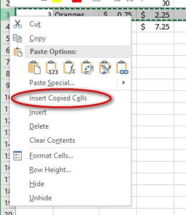
We need to add “Mandarin Oranges” to the list. The long way would be to right-click “Copy Row 3,” then right-click “Insert Row,” then type and copy our formulas. Instead, let’s right-click “Copy Row 3,” then stay on Row 3, and right-click “Insert Copied Cells.” This will insert a new Row 4 with the same information already found in Row 3.
When you copy and paste, Excel keeps our formulas “relative” to their rows: the Row 3 formulas use Row 3 cells, and the Row 4 formulas use Row 4 cells. Click on “Show Formulas” if you’d like to see this for yourself. Then click off “Show Formulas” and return to our Home tab.
Tip: Always click back on the “Home” tab after finishing with another tab, especially if you’re a beginner.
Edit Cells
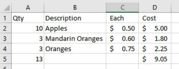
We now have two rows of “Oranges.” Let’s change Row 3. Click on the word “Oranges” in Cell B3, and change it to “Mandarin Oranges” by either editing the cell or typing the new words over the old. “Mandarin Oranges” doesn’t quite fit in Column B, so double-click between “B” and “C” to extend the column width.
Change the price of these smaller oranges to 60-cents by changing the “.75” to “.6” instead. Notice that the cell formatting stays the same, and “.6” changes to “$0.60.”
Do you notice a problem with the total in our “quantity” column? Remember our “quantity” column added together the number of apples sold to the number of oranges sold. Since that quantity is only adding two numbers, it does not include the “Mandarin Oranges.” Click on Cell A5 and then click in the Formula Bar, and you’ll see Excel’s colors showing you Cell A3 is not included in the sum.
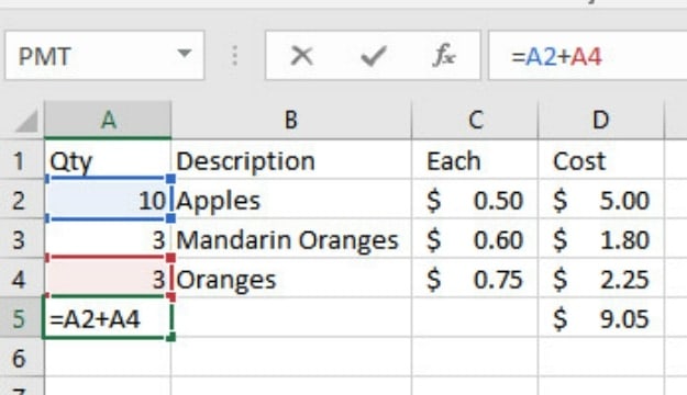
Our total cost in Cell D5 is correct because it is adding up or finding the “sum” of a range of numbers using the “=SUM()” formula. When we added a row, Excel extended the range to include those numbers. Click on Cell D5, then click in the formula bar to see.

Format As Table
Excel has a shortcut to place your data in Table Format to make sums much easier. Click on Row 5, then right-click “Delete” to remove the old sums. You may also click on Row 5 and hit the “Delete” button, or delete them one at a time. Remember, there is usually more than one correct way to do things in MS Office.
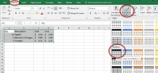
Starting with our top left heading, drag through all the data, from Cell A1 to Cell D4. On the “Home tab>Styles Section>click Format as Table.” Microsoft has created many table formatting options to choose from. My favorite is the black header with grey and white rows in the “Medium” section, but you may choose your favorite.
Pro Tip: If you are going to print your table, stay away from the dark section, it uses quite a bit of costly ink.
The “Format as Table” window will appear to confirm your data. In the window, “My table has headers” is checked. Excel saw the word descriptions of each column at the top of our table, so it will use those as headers if the box remains checked. Click “OK” and watch what happens.
Our little list of data is now a neat little Excel table.

Totals Row
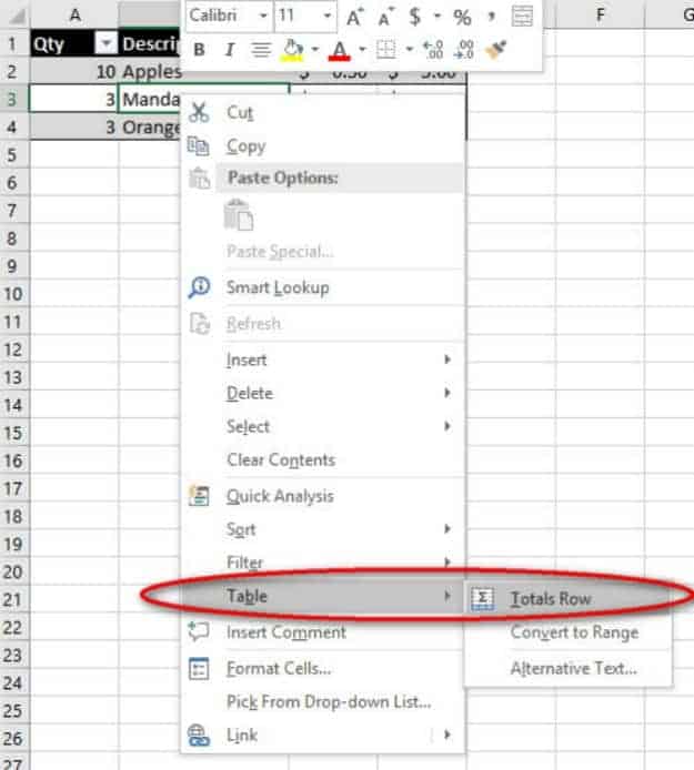
Right-click any cell inside the table. Near the bottom of this pop-up menu, point to “Table” and more selections will appear. Right-click “Table>Totals Row.”
Excel creates a special row at the bottom which adds up the right-hand column automatically. Click on the total in Column D and a small drop-down arrow appears. Click the drop-down arrow, and you will see many different formulas are available, such as average, minimum, and maximum.
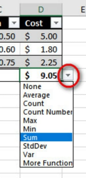
Table Sort
Do you see the drop-down arrows in the top row? These are sort and filter options. Click on the “Description” drop-down arrow. There are A-Z and Z-A sorting options and filtering choices. Sort our fruit Z-A to change the order. The prices stay with each fruit, and the totals stay the same. Now sort the price smallest to largest. Are the totals affected? Nope.
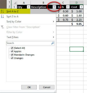
Table Filter
Let’s see how much money we made on just our oranges, both mandarin and regular. Click the “Description” drop-down arrow and go to the “Text Filter” section. Do you see all our descriptions listed in alphabetical order? Now, start typing “orange” in the text filter box, and all our oranges are checked.

You didn’t need to type “Oranges” just any part of the word in lower case like “orange.” As you typed, Excel “filtered” out the words that didn’t match. Look at your total. Your total changed to just show the cost of all the oranges.
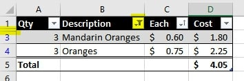
Excel signals you that the table is filtered and some of the data is not showing. First, notice that a small funnel has replaced the description drop-down arrow. Second, notice that row 2 is missing and has been replaced by a double line between the “1” and the “3.” I’d recommend never saving a table that has an active filter because you’ll forget that not all your information is there.
Select All
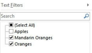
How do we get our data back? Click the small funnel. “Mandarin Oranges” is checked, “Oranges” is checked, but “Apples” is unchecked. The “Select All” box is blackened because not all the items are selected. Click on the “Select All” box so it is checked. When you click “OK,” your “apples” row will reappear, and your total will reflect all your sales.
Practice
Add a few more rows, and sort each of your table’s columns for practice. Play around with the number formats, check the options in the drop-down list, or experiment with the format code. Filter out one or two of the rows. You may type part of the word to be filtered, or uncheck the little boxes – whichever is easiest. Sometimes the size and type of data makes one way easier than another BUT always go back to “Select All” before saving.
What was the most helpful part of this lesson? Let us know in the comments below!